Automated assessment of residual plots with computer vision models

ASC2025 talk

Patrick Li

RSFAS, ANU

About me

Hi! I am Patrick Li.

I completed my PhD in Statistics at EBS, Monash University. My research focused on computer vision and data visualization, with an emphasis on developing visual analytics methods to assess residual plots.
I am a postdoctoral researcher at ANU contributing to the Analytics for the Australian Grains Industry (AAGI) project, where my work centres on machine learning, image analytics, and plant phenotyping.

️Co-authors

Prof Dianne Cook

Department of Econometrics and Business Statistics, Melbourne, Monash University

Dr. Emi Tanaka

Research School of Finance, Actuarial Studies and Statistics, Australian National University

Asst Prof Susan VanderPlas

Statistics Department, University of Nebraska-Lincoln

A/Prof Klaus Ackermann

Department of Econometrics and Business Statistics, Melbourne, Monash University, Australia

Challenges in interpreting residual plots reliably

Residual plot of a simple linear regression:

Challenges in interpreting residual plots reliably

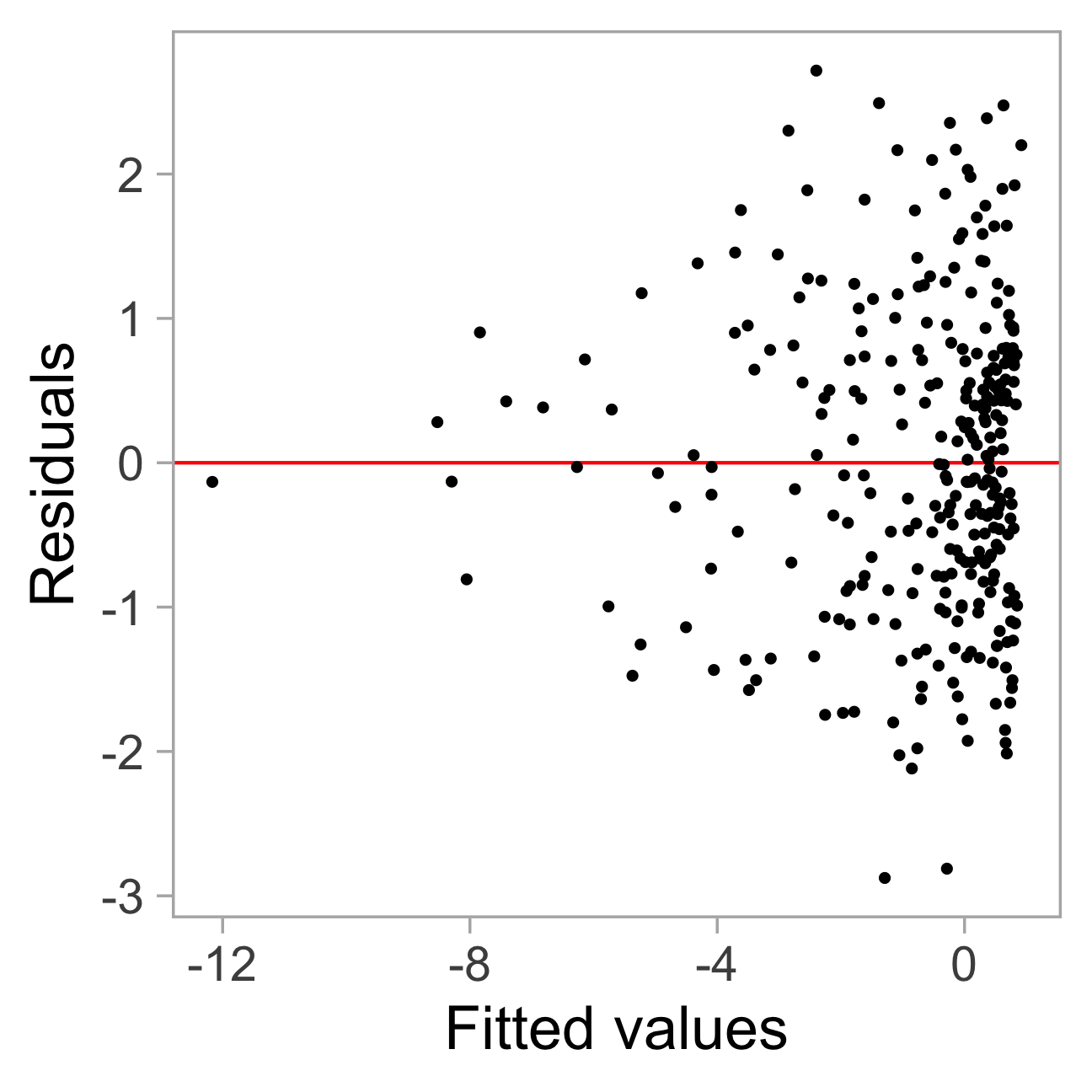
Residual plot of a simple linear regression:

Heteroskedasticity: Vertical spread of the points varies with the fitted values.
However, this is an over-interpretation.
The visual pattern is caused by a skewed distribution of the predictor.

Validity of visual discoveries

Visual discoveries that may appear to violate model assumptions:

Random variation or sampling noise
Features of the predictors
> Genuine model-assumption violations
…

How do we determine which visual discoveries are valid?

Visual inference (Buja, et al. 2009)

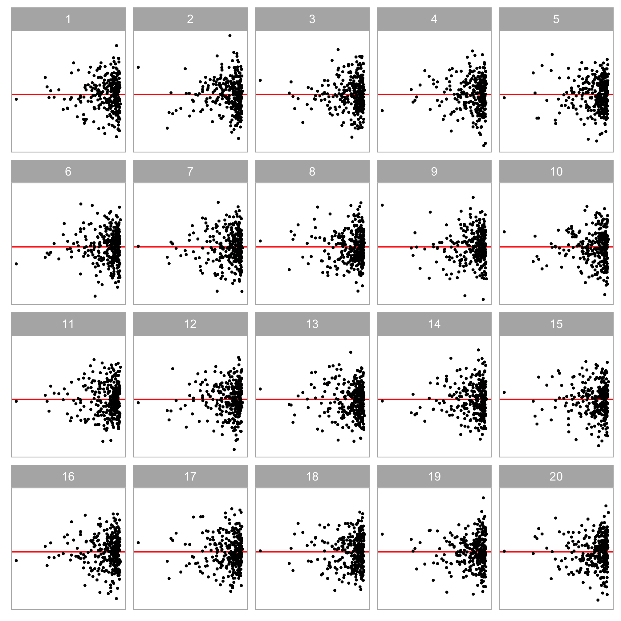
Visual discoveries can be validated by an inferential framework called visual inference.

A lineup of residual plots:

1 actual residual plot
19 null plots containing residuals simulated from the fitted model.

To perform a visual test:

Ask observer(s) to pick the most different plot(s).
Calculate the p-value using the beta-binomial model (VanderPlas et al., 2021).

Null residuals simulation (Buja, et al. 2009)

For a classical normal linear regression model:

\hat{\boldsymbol{\beta}} = (\boldsymbol{X}^\top\boldsymbol{X})^{-1}\boldsymbol{X}^\top\boldsymbol{y},\quad \hat{\sigma}^2 = \frac{(\boldsymbol{y} - \boldsymbol{X}\boldsymbol{\beta})'(\boldsymbol{y} - \boldsymbol{X}\boldsymbol{\beta})}{n-p}.

Simulate \tilde{\boldsymbol{e}} \sim N(\boldsymbol{0}, \hat{\sigma}^2\boldsymbol{I})
Obtain \tilde{\boldsymbol{y}} = \boldsymbol{X}\hat{\boldsymbol{\beta}} + \tilde{\boldsymbol{e}}
Estimate \tilde{\boldsymbol{\beta}} = (\boldsymbol{X}^\top\boldsymbol{X})^{-1}\boldsymbol{X}^\top\tilde{\boldsymbol{y}}
Obtain \boldsymbol{e}_{null} = \tilde{\boldsymbol{y}} - \boldsymbol{X}\tilde{\boldsymbol{\beta}}, \quad\hat{\boldsymbol{y}}_{null} = \boldsymbol{X}\tilde{\boldsymbol{\beta}}

Characteristics of the lineup protocol

✅

All-in-one test: can detect many visually recognisable violations
Validated visual findings: helps identify which visual patterns are truly meaningful and may guide model refinement.

❌

Human constraints:
- hard to evaluate many lineups
- hard to process lineups with many plots
Resource-intensive: high labour cost and time-consuming

Can we automate it?

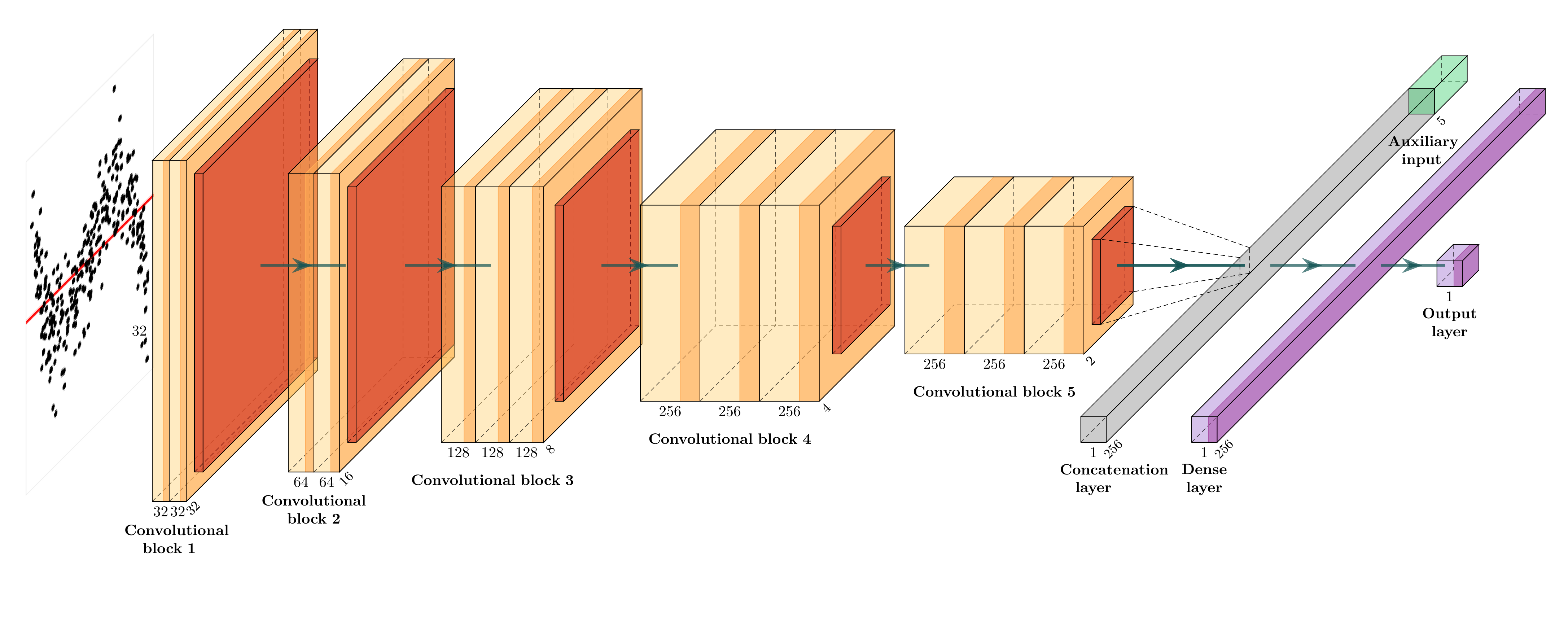
Computer vision model

Modern computer vision models are well-suited for addressing this challenge.

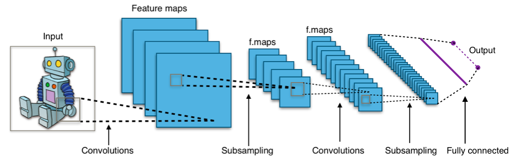
Source: https://en.wikipedia.org/wiki/Convolutional_neural_network

Measure the difference

How do we define a numerical measure of “difference” or “distance” between plots?

pixel-wise sum of square differences?
Structural Similarity Index Measure (SSIM)?
scagnostics?
…

Distance from a “theoretically” good residual plot

We defined a distance measure based on Kullback-Leibler divergence to quantify the extent of model violations:

D = \log\left(1 + \int_{\mathbb{R}^{n}}\log\frac{p(\boldsymbol{e})}{q(\boldsymbol{e})}p(\boldsymbol{e})d\boldsymbol{e}\right).

P: reference residual distribution assumed under correct model specification.
Q: actual residual distribution.
D = 0 if and only if P \equiv Q.

However, Q is unknown in practice \Rightarrow D can not be computed.

Simulation of training data

In a simulation, we can control the data-generating process and therefore know the true residual distribution Q.

Non-linearity + Heteroskedasticity

Non-normality + Heteroskedasticity

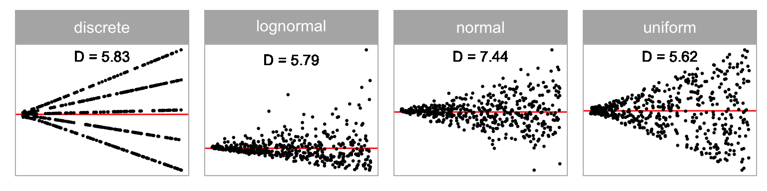
Distribution of predictor

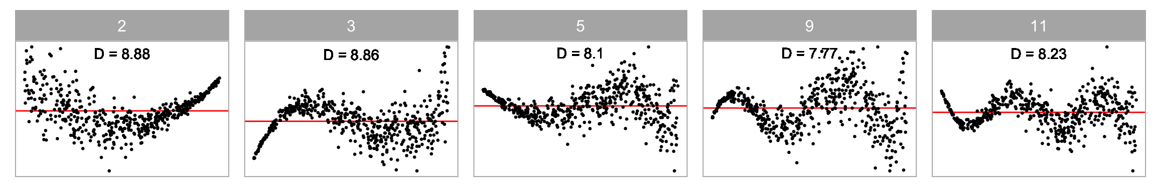
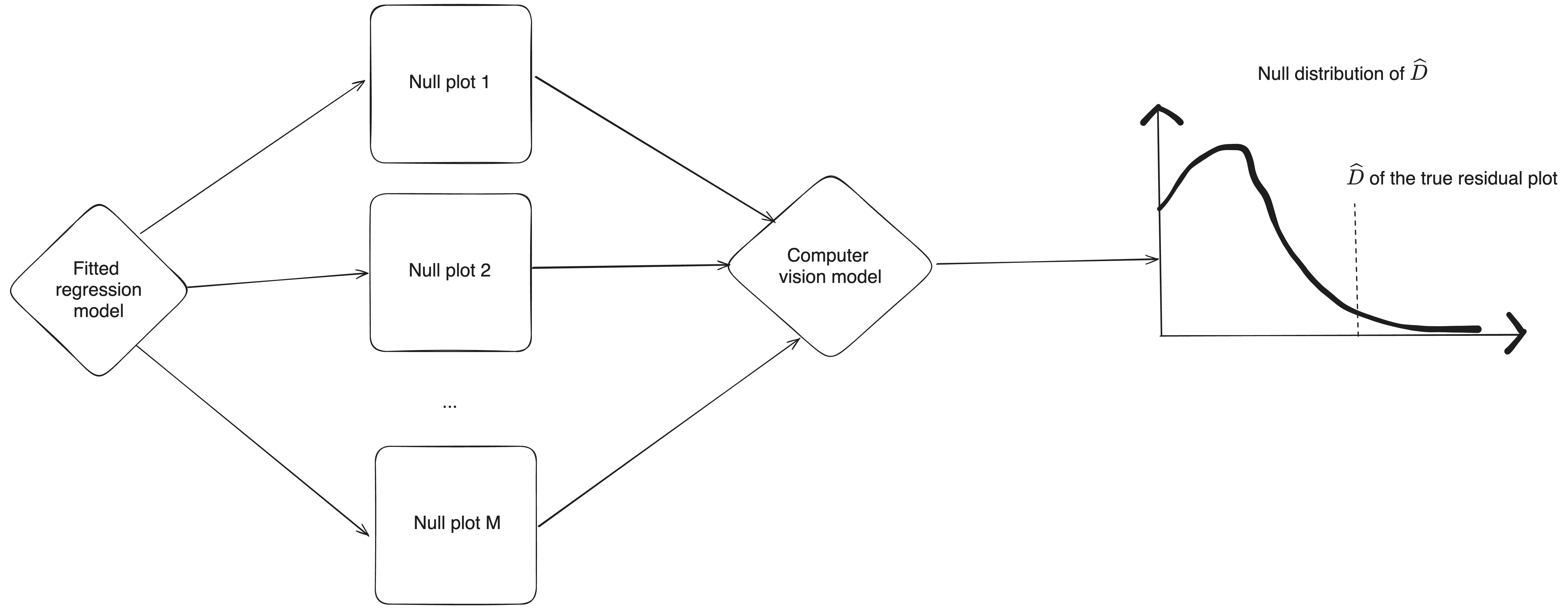
Estimation of D

We train a computer vision model to estimate D with 64,000 simulated residual plots:

\widehat{D} = f_{CV}(V_{h \times w}(\boldsymbol{e}, \boldsymbol{\hat{y}})),

where V_{h \times w}(.) generates an h \times w image, and f_{CV}(.) predicts a non-negative distance.

Statistical testing

The p-value is the proportion of null plots having \widehat{D} greater than or equal to the observed one.

`autovi` Package

Li, W., Cook, D., Tanaka, E., VanderPlas, S., & Ackermann, K. (2025). Automated Residual Plot Assessment With the R Package autovi and the Shiny Application autovi. web. Australian & New Zealand Journal of Statistics.

Core Methods

Null residuals simulation: rotate_resid()
Visual signal strength (\widehat{D} prediction): vss()
Comprehensive checks: check() and summary_plot()

Example: Boston housing

library(autovi)
fitted_model <- lm(MEDV ~ RM + LSTAT + PTRATIO, data = housing)
checker <- residual_checker(fitted_model)
checker$plot_resid()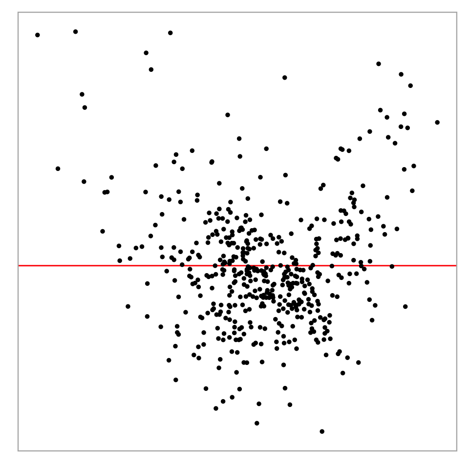

`rotate_resid()`

Null residuals are simulated from the fitted model assuming it is correctly specified.

checker$rotate_resid()

# A tibble: 489 × 2
   .fitted   .resid
     <dbl>    <dbl>
 1 632372.   82404.
 2 525177.   24363.
 3 646753.  -16642.
 4 624848.    7895.
 5 611817.  -25387.
 6 551051. -128980.
 7 504757.  -37748.
 8 445700.   33616.
 9 281912.  -17081.
10 453398. -103580.
# ℹ 479 more rows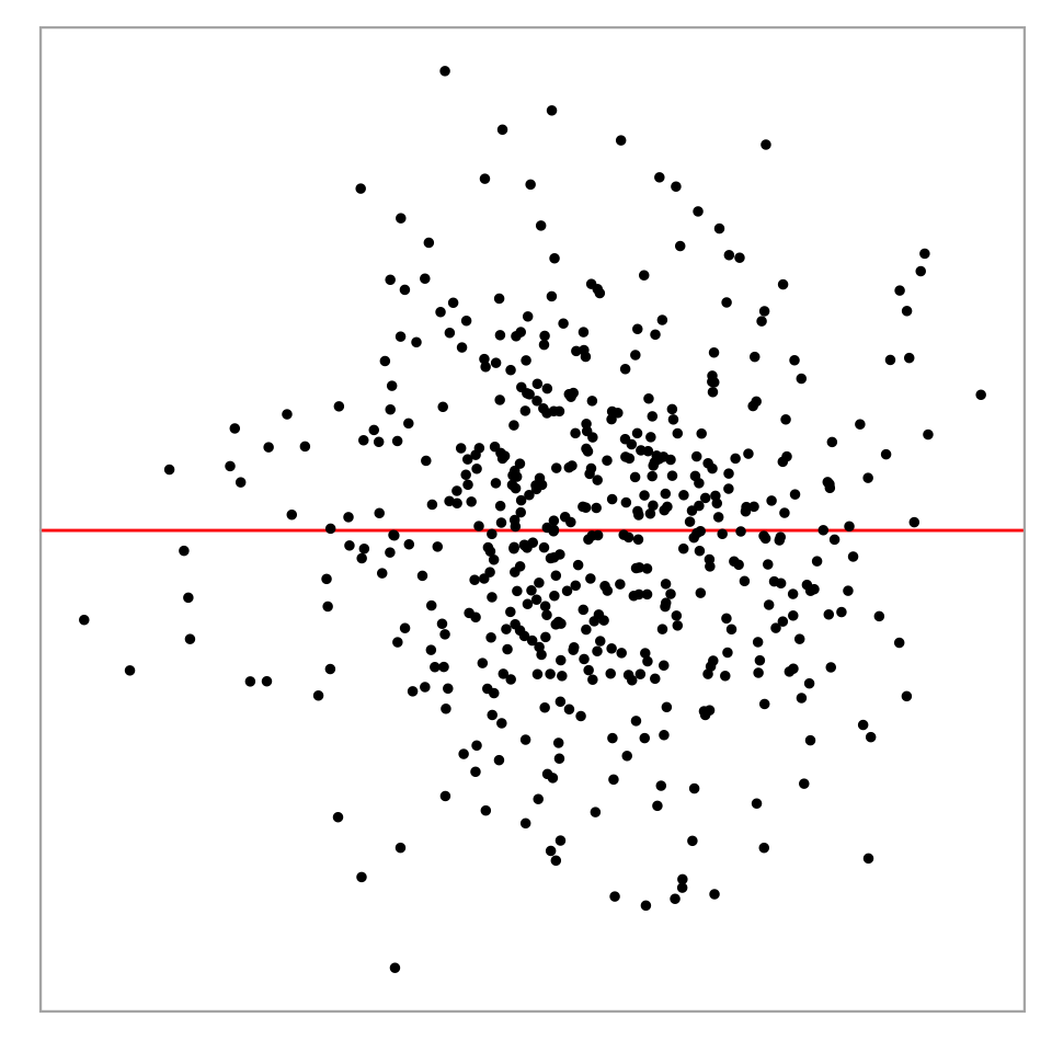

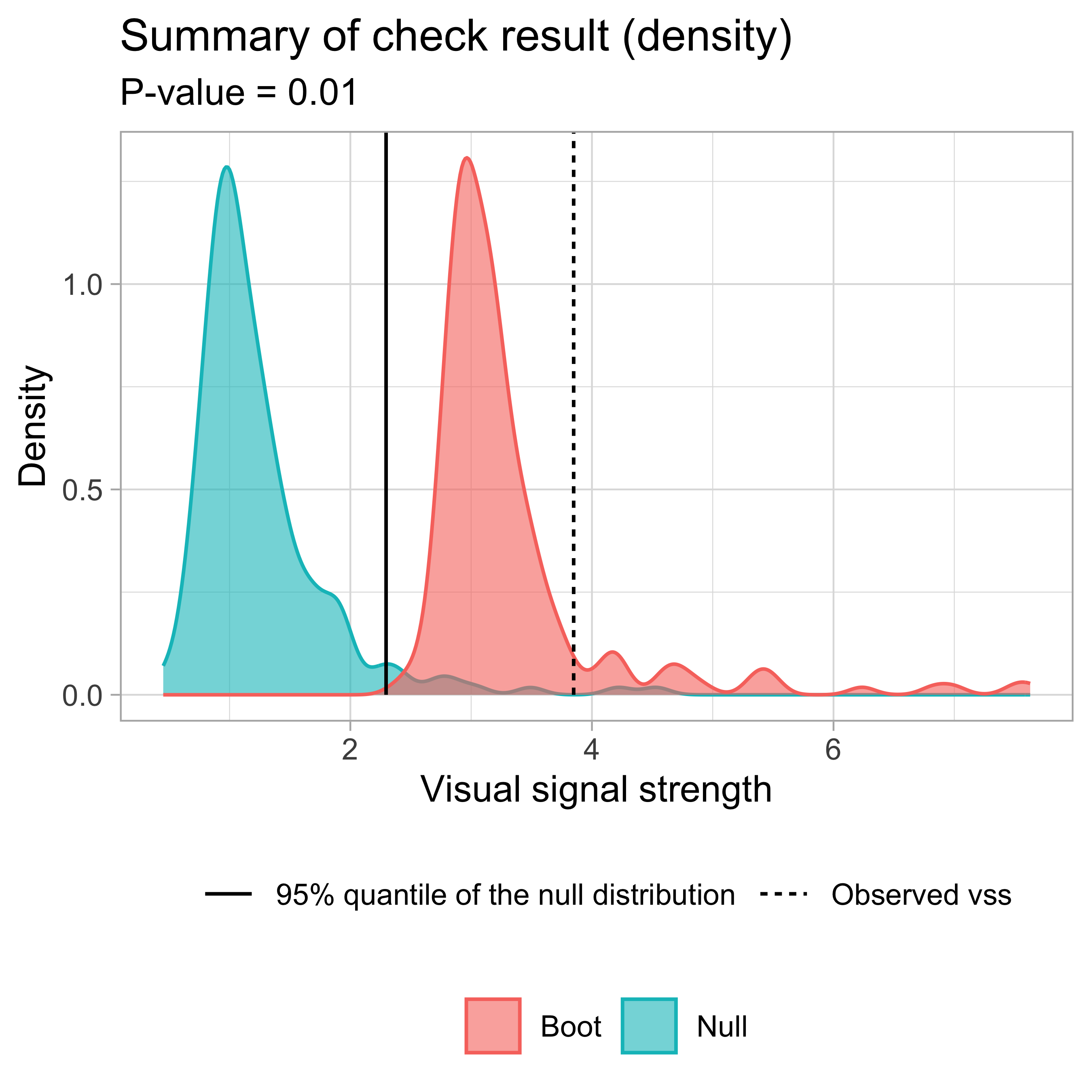
checker$rotate_resid() |>
  checker$plot_resid()

`vss()`

Visual signal strength \widehat{D} of the actual residual plot

checker$vss()

✔ Predict visual signal strength for 1 image.

# A tibble: 1 × 1
    vss
  <dbl>
1  6.48

Visual signal strength \widehat{D} of a null plot

checker$rotate_resid() |>
  checker$vss()

✔ Predict visual signal strength for 1 image.

# A tibble: 1 × 1
    vss
  <dbl>
1  1.26

`check()` and `summary_plot()`

checker$check()

── <AUTO_VI object>
Status:
 - Fitted model: lm
 - Keras model: (None, 32, 32, 3) + (None, 5) -> (None, 1)
    - Output node index: 1
 - Result:
    - Observed visual signal strength: 6.484 (p-value = 0)
    - Null visual signal strength: [100 draws]
       - Mean: 1.169
       - Quantiles: 
          ╔══════════════════════════════════════════╗
          ║  25%   50%   75%   80%   90%   95%   99% ║
          ║1.037 1.120 1.231 1.247 1.421 1.528 1.993 ║
          ╚══════════════════════════════════════════╝
    - Bootstrapped visual signal strength: [100 draws]
       - Mean: 6.28 (p-value = 0)
       - Quantiles: 
          ╔══════════════════════════════════════════╗
          ║  25%   50%   75%   80%   90%   95%   99% ║
          ║5.960 6.267 6.614 6.693 6.891 7.112 7.217 ║
          ╚══════════════════════════════════════════╝
    - Likelihood ratio: 0.7064 (boot) / 0 (null) = Extremely large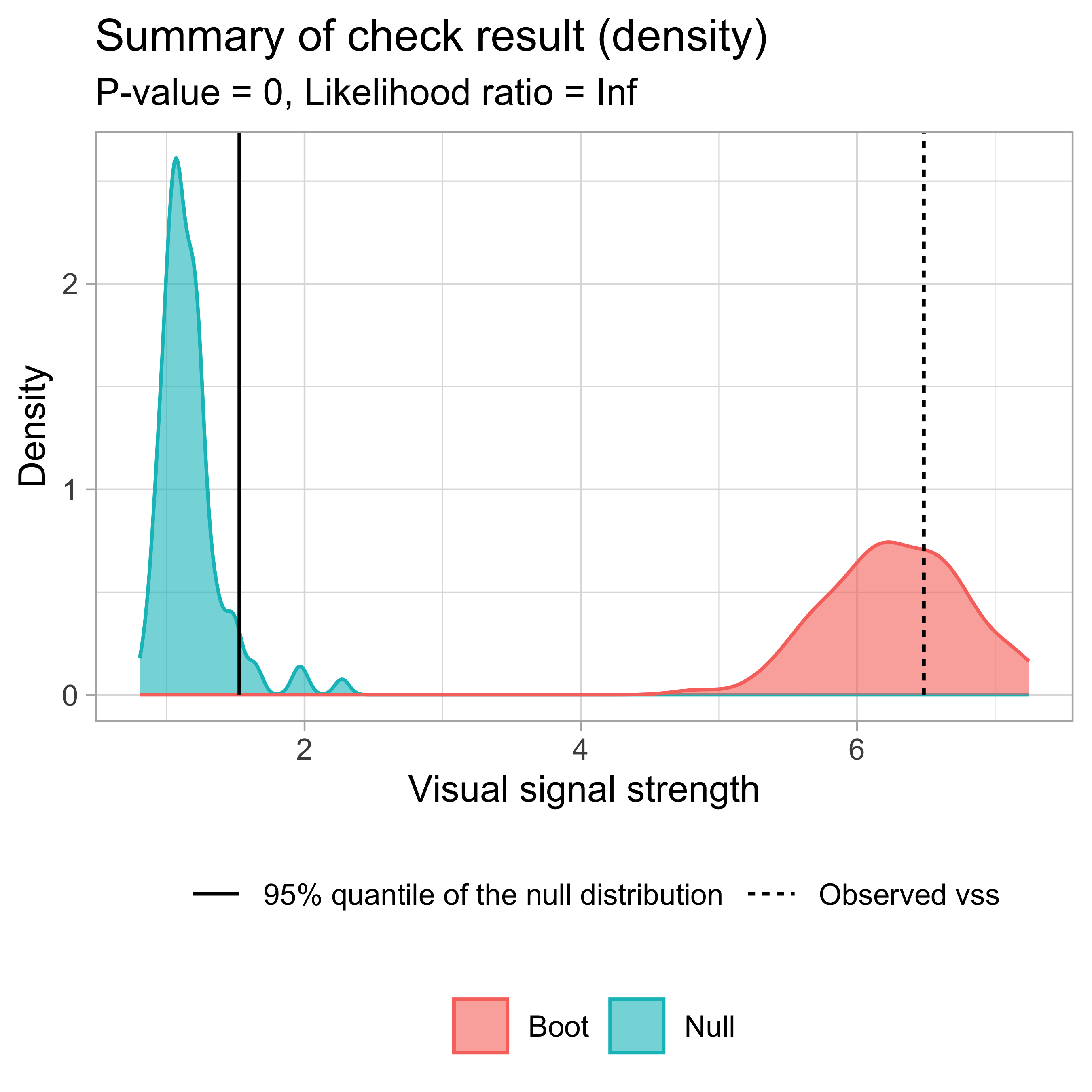

checker$summary_plot()

Example: Left-triangle

Breusch–Pagan test p-value = 0.0457

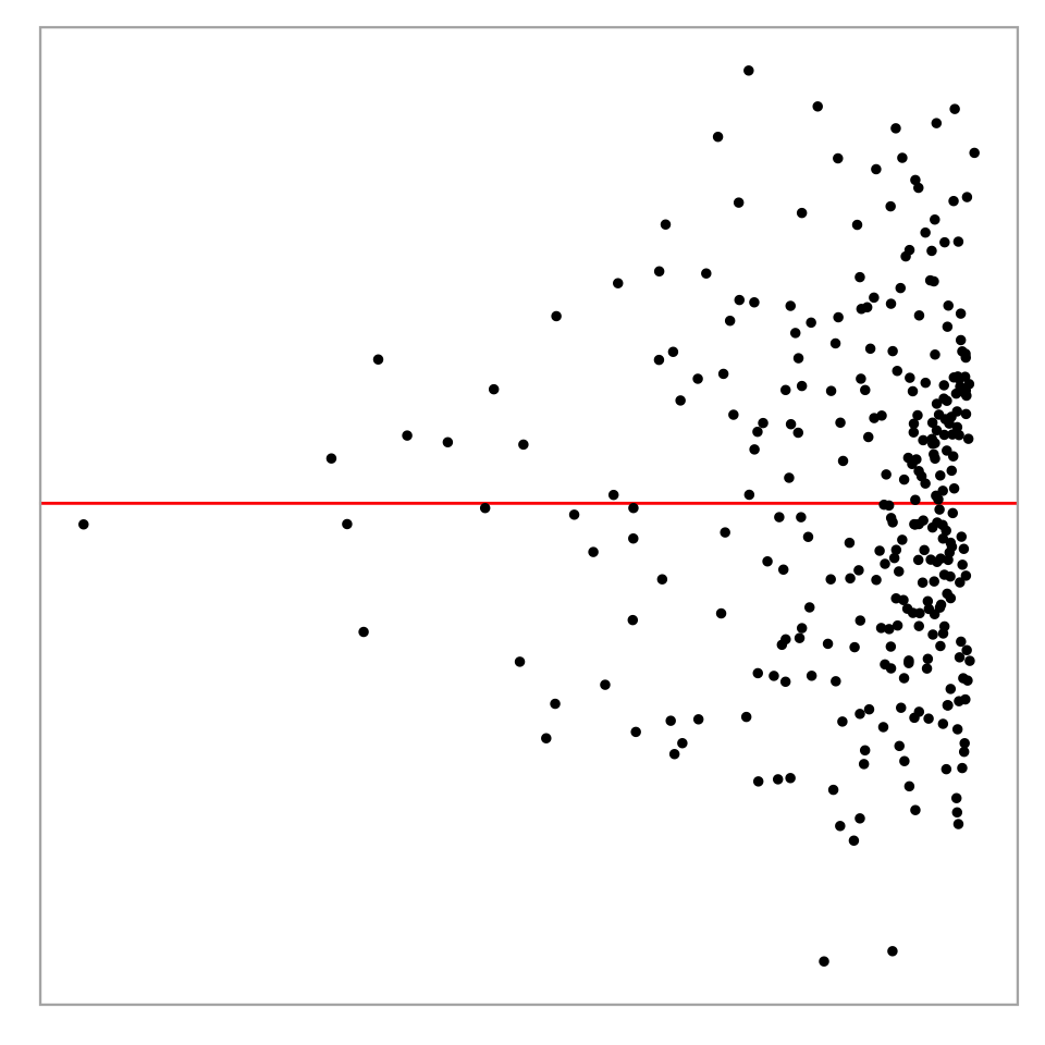
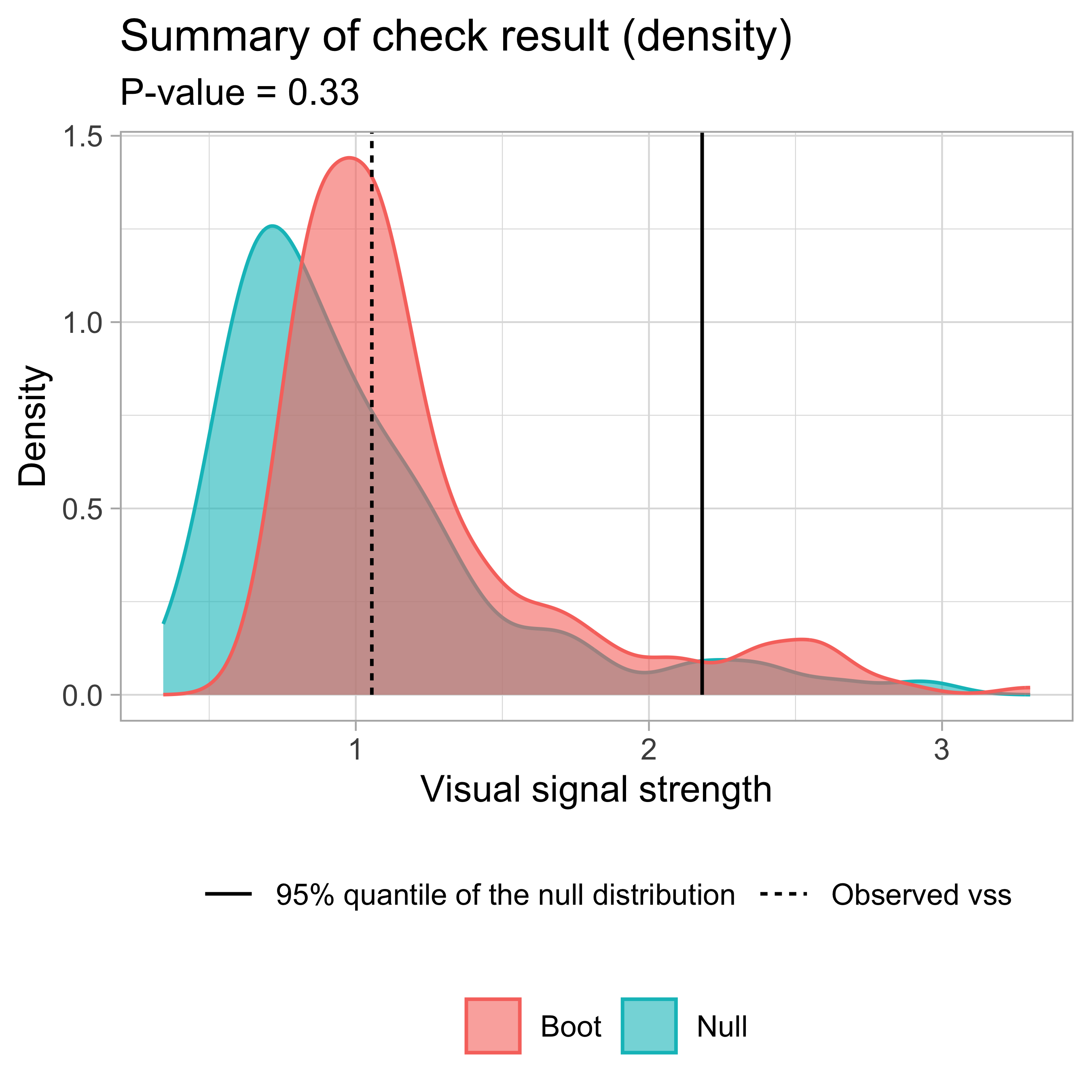
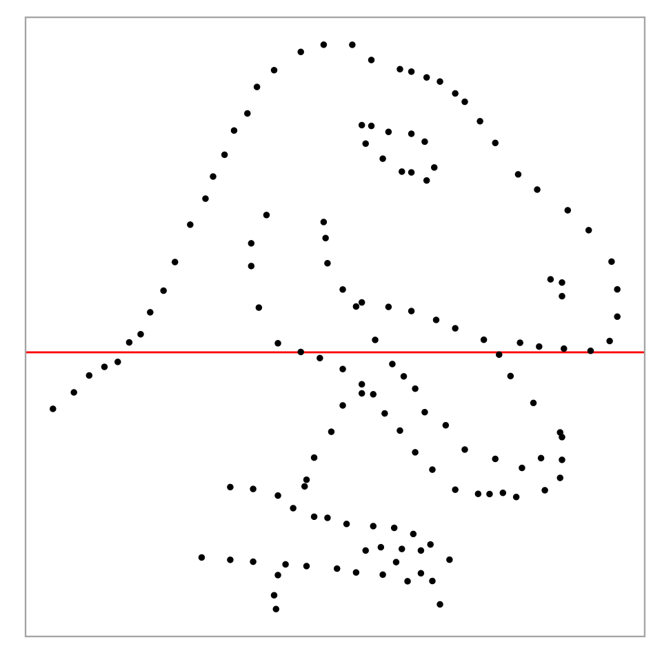
💡Example: Dinosaur

Ramsey Regression Equation Specification Error test p-value = 0.742

Breusch–Pagan test p-value = 0.36

Shapiro-Wilk test p-value = 9.21e-05

🌐Shiny Application

Don’t want to install TensorFlow?

Try our shiny web application: http://autovi.patrickli.org/

Takeaway

You can use autovi to

Evaluate lineups of residual plots of linear regression models
Captures the extent of model violations through visual signal strength
Automatically detect model misspecification using a visual test

Research on extensions to GLM and LMM frameworks is still in progress.

Thanks! Any questions?

Li, W., Cook, D., Tanaka, E., VanderPlas, S., & Ackermann, K. (2024). Automated Assessment of Residual Plots with Computer Vision Models. arXiv preprint arXiv:2411.01001.

tengmcing

[email protected]

📦 https://github.com/TengMCing/autovi

📜 https://github.com/TengMCing/asc2025-autovi